
MLOps Project, Part 4a: Machine learning model monitoring
 Isaac Kargar7 min read
A prediction service can return successful HTTP responses while its predictions become less useful. A schema change, a missing input field, or a different mix of customers can affect the model without taking the endpoint offline. After deploying a model, we need to watch the data and outcomes as well as the service.
This post compares two subsets of the California Housing dataset with Evidently, then uses Alibi Detect to show how numerical and categorical drift tests work together. The examples run locally and do not require a hosted monitoring account.
What to monitor
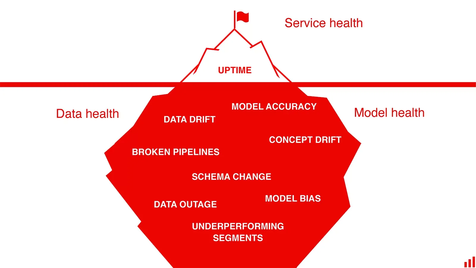
| Layer | Useful signals | What a change can mean |
|---|---|---|
| Service | Error rate, latency, resource use, failed dependencies | The application cannot reliably process requests |
| Data quality | Missing values, types, ranges, duplicate records, fresh inputs | A collection or transformation step may be broken |
| Data distribution | Feature, prediction, and target distributions | The current population differs from the reference population |
| Model quality | Error against observed outcomes, calibration, performance by segment | Predictions may no longer meet the task’s requirements |
Data drift is a change in the input distribution. Concept drift is a change in the relationship between inputs and the outcome. Neither follows automatically from a single monitoring alert. A geographic shift in housing data, for example, may change the price distribution while a model that uses location still predicts well.
Prediction drift can be measured before labels arrive. Prediction quality needs observed outcomes: classification labels, actual prices, or another task-specific target. Label delays and missing labels matter because the evaluated subset may differ from all requests.
Compare two datasets with Evidently
Evidently reports combine metrics and presets over a dataset. A drift report needs a reference dataset and a current dataset. Map their columns consistently so a numeric identifier is not accidentally treated as a continuous measurement.
Use Python 3.12 and these package versions for the examples:
python3.12 -m venv .venv
source .venv/bin/activate
python -m pip install evidently==0.7.21 alibi-detect==0.13.0 \
  scikit-learn==1.9.0 pandas==2.3.3 numpy==1.26.4 scipy==1.17.1
California Housing contains eight input features and the target MedHouseVal. We take 1,000 rows from the first 15,000 records as the reference and 1,000 from the remaining records as the comparison. This is a comparison between dataset subsets, not evidence of temporal drift in a deployed housing model.
from sklearn.datasets import fetch_california_housing
from evidently import DataDefinition, Dataset, Report
from evidently.presets import DataDriftPreset

housing = fetch_california_housing(as_frame=True)
frame = housing.frame
columns = frame.columns.tolist()

reference_frame = frame.iloc[:15000].sample(1000, random_state=0)
current_frame = frame.iloc[15000:].sample(1000, random_state=0)

definition = DataDefinition(numerical_columns=columns)
reference = Dataset.from_pandas(reference_frame, data_definition=definition)
current = Dataset.from_pandas(current_frame, data_definition=definition)

report = Report([
    DataDriftPreset(
        columns=columns,
        method="ks",
        threshold=0.05,
        drift_share=0.5,
    )
])
result = report.run(current_data=current, reference_data=reference)
result.save_html("housing-drift.html")
result.save_json("housing-drift.json")
The first run downloads the public dataset. Open housing-drift.html to inspect distributions and the report’s column-level results. The JSON file contains the corresponding machine-readable results. The data definition guide explains how to map targets, predictions, categories, and text for other reports.
We explicitly select the two-sample Kolmogorov-Smirnov test rather than relying on automatic test selection. It compares the empirical cumulative distributions of a numerical column. At the chosen per-column threshold of 0.05, seven of the nine monitored columns are flagged:
| Column | K-S p-value, rounded | Drift at 0.05 |
|---|---|---|
| MedInc | 0.000348 | Detected |
| HouseAge | 0.00000175 | Detected |
| AveRooms | 0.001449 | Detected |
| AveBedrms | 0.465960 | Not detected |
| Population | 0.500567 | Not detected |
| AveOccup | 0.004544 | Detected |
| Latitude | 3.41e-100 | Detected |
| Longitude | 2.92e-125 | Detected |
| MedHouseVal | 6.98e-13 | Detected |
That is 77.78% of the monitored columns, which includes the target. It is not seven of eight input features. The dataset-level flag also fires because the share exceeds the configured 50% threshold. Evidently’s drift preset documentation describes this aggregation and the available test choices.
A p-value displayed as 0.000000 can be a rounded very small value. It is not a probability that the datasets are identical, nor a measure of the business impact of the shift. Check the distributions, sample sizes, and affected segments before deciding what to do. Testing many columns also increases the chance of a false alert; the per-column tests above do not apply a multiple-testing correction.
Drift tests do not replace quality checks. Missing values, invalid categories, and delayed records deserve separate checks because a distribution test may operate only on the nonmissing values. If actual sale prices become available, compare predictions with those prices to measure model error directly.
Numerical and categorical drift with Alibi Detect
Alibi Detect provides detectors for distribution changes, outliers, and adversarial inputs. These ask different questions. An outlier detector scores an individual observation against its reference behavior; a drift detector usually compares batches or monitors a stream for a distribution change.
For mixed tabular data, TabularDrift combines K-S tests for numerical columns with chi-squared tests for categorical columns. The category mapping tells it which positions in the input array represent categories. The TabularDrift API reference documents that mapping and its multiple-testing options.
The next example uses income and house age from the same housing samples. It adds a binary longitude band solely to demonstrate categorical handling: 1 means longitude is below -120, and 0 means it is not.
import numpy as np
from alibi_detect.cd import TabularDrift


def mixed_features(data):
    return np.column_stack([
        data["MedInc"].to_numpy(),
        data["HouseAge"].to_numpy(),
        (data["Longitude"] < -120).astype(int).to_numpy(),
    ])


feature_names = ["MedInc", "HouseAge", "Longitude below -120"]
detector = TabularDrift(
    mixed_features(reference_frame),
    p_val=0.05,
    categories_per_feature={2: 2},
    correction="bonferroni",
)
drift = detector.predict(mixed_features(current_frame))["data"]

print("Dataset drift:", bool(drift["is_drift"]))
print("Corrected threshold:", drift["threshold"])
for name, p_value in zip(feature_names, drift["p_val"]):
    print(name, f"p={p_value:.6g}")
The detector flags a shift in this comparison. With three tested columns, the Bonferroni threshold is 0.05 / 3, or approximately 0.0167. Bonferroni controls the family-wise probability of at least one false rejection under the test assumptions. False-discovery-rate procedures instead control an expected proportion of false discoveries among rejections. These are different objectives, so choose the correction before interpreting alerts.
The test should also match the type and structure of the data:
| Method | What it compares | A limit to consider |
|---|---|---|
| K-S test | Two univariate numerical distributions | Separate feature tests can miss a change in dependence between features |
| Chi-squared test | Category frequencies | Sparse expected counts can make the approximation unsuitable |
| Fisher’s exact test | A contingency table, such as counts for a binary outcome in two batches | A binary test does not directly handle arbitrary continuous measurements |
| Maximum mean discrepancy | Multivariate distributions through a kernel | Kernel choice, representation, and sample size affect sensitivity |
| Learned-kernel test | Distributions using a kernel fitted to distinguish them | Kernel fitting and the final test need appropriate data separation |
Alibi also includes outlier methods such as autoencoders, autoencoding mixture models, and time-series detectors. An autoencoder uses reconstruction error, while a forecasting detector compares observations with its expected range. Those scores need calibration on data representing acceptable behavior. A reconstruction error alone does not establish that an input is malicious.
Run monitoring around the prediction service
Keep monitoring work outside the request’s critical path. Record enough information to join a prediction with its later outcome, then evaluate bounded batches on a schedule. Restrict access and retention for captured inputs because monitoring data can contain the same sensitive fields as inference traffic.
A practical sequence is:
- Choose a reference period and record which population it represents.
- Capture input-quality statistics, predictions, timestamps, and the model version used.
- Compare a current window with an appropriate reference window, accounting for seasonality and segment size.
- Join delayed outcomes when they arrive and measure prediction error on the labelled subset.
- Route alerts to an owner who can investigate the data pipeline, serving changes, and model behavior.
Managed services can handle parts of this workflow. Existing users of Amazon SageMaker Model Monitor can capture inference data, run baseline comparisons on a schedule, and send metrics to CloudWatch. AWS no longer accepts new customers for that service. Its data-quality checks and its model-quality checks use different inputs: measuring prediction quality requires outcomes joined to the predictions.
A drift alert should start an investigation. If a schema bug caused the shift, fix the pipeline. If the population changed but prediction quality remains acceptable, retraining may not help. When a model change is warranted, evaluate the candidate against the current model and the affected segments before replacing it. Monitoring is useful when its signals lead to a specific, checkable action.
Work with Nazmi
Build your AI system with Nazmi.
Tell us what you are building, what exists today, and where your team needs help.
Start a conversation or book a 20-minute call →