Data Engineering — Week 3a: Data Warehouse

Week 3 — Data Engineering Zoomcamp course: Data Warehouse

Note: The content of this post is from the course videos, my understanding and searches, and reference documentation.

Data Warehouse

OLTP vs OLAP

The two terms look similar but refer to different kinds of systems. Online transaction processing (OLTP) captures, stores, and processes data from transactions in real-time. Online analytical processing (OLAP) uses complex queries to analyze aggregated historical data from OLTP systems.

An OLTP system is a database that captures and retains transaction data. Individual database entries made up of numerous fields or columns are involved in each transaction. Banking and credit card transactions, as well as retail checkout scanning, are examples. Because OLTP databases are read, written, and updated frequently, the emphasis in OLTP is on fast processing. Built-in system logic protects data integrity if a transaction fails.

For data mining, analytics, and business intelligence initiatives, OLAP applies complicated queries to massive amounts of historical data aggregated from OLTP databases and other sources. The emphasis in OLAP is on query response speed for these complicated queries. Each query has one or more columns of data derived from a large number of rows. Financial performance year over year or marketing lead generation trends are two examples. Analysts and decision-makers can utilize custom reporting tools to turn data into information using OLAP databases and data warehouses. OLAP query failure does not affect or delay client transaction processing, but it can affect or delay the accuracy of business intelligence insights. [ ref]

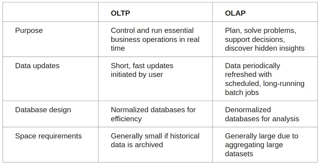
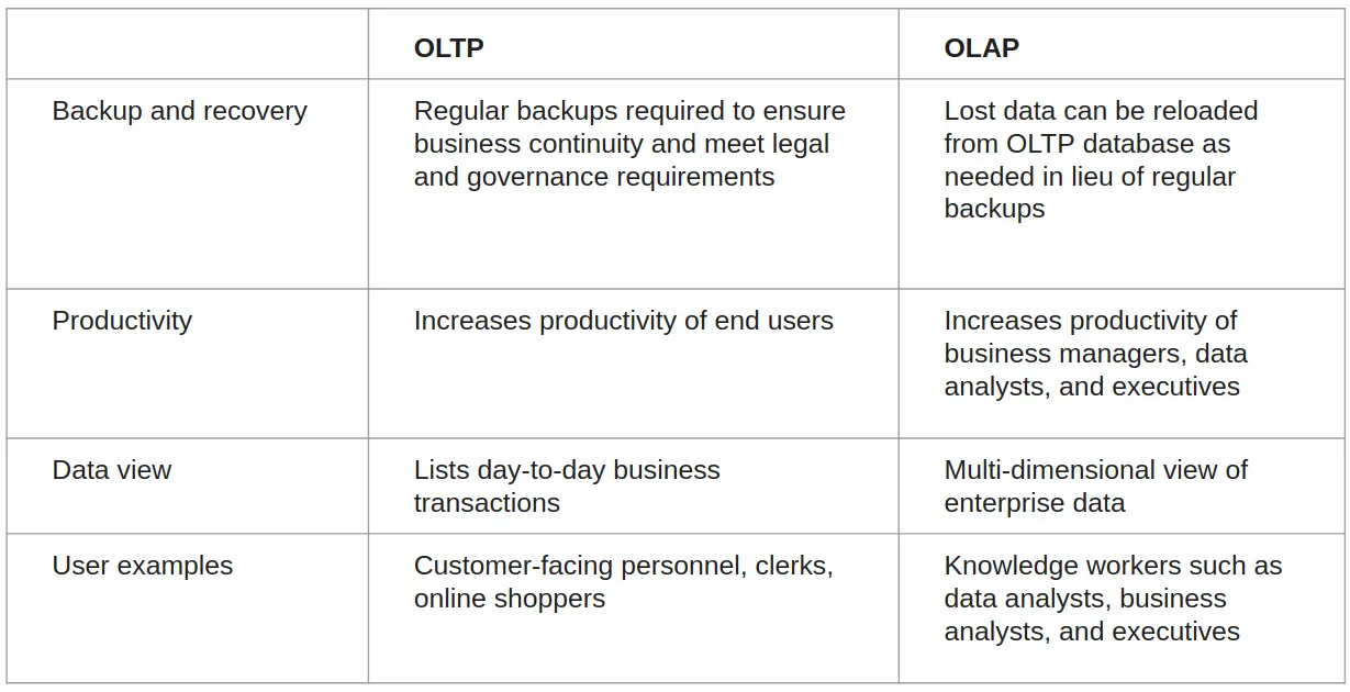
Data Warehouse

DE Zoomcamp 3.1.1 - Data Warehouse and BigQuery

A data warehouse (DW or DWH), often known as an enterprise data warehouse (EDW), is a reporting and data analysis system that is considered a key component of business intelligence. DWs are central data repositories that combine data from a variety of sources. They keep current and historical data in one place and utilize it to generate analytical reports for employees across the company.

The data in the warehouse comes from the operating systems and is uploaded there (such as marketing or sales). Before being used in the DW for reporting, the data may transit via an operational data store and require data cleansing for extra procedures to ensure data quality.

The two major methodologies used to design a data warehouse system extract, transform, load (ETL), and extract, load, transform (ELT). [ wikipedia]

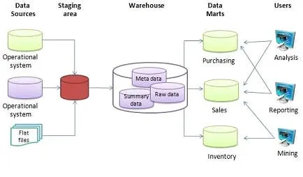
Google BigQuery, Amazon Redshift, and Microsoft Azure Synapse Analytics are three data warehouse services. Here we review BigQuery and Redshift.

BigQuery

BigQuery is a fully managed enterprise data warehouse that helps you manage and analyze your data with built-in features like machine learning, geospatial analysis, and business intelligence. BigQuery’s serverless architecture lets you use SQL queries to answer your organization’s biggest questions with zero infrastructure management. BigQuery’s scalable, distributed analysis engine lets you query terabytes in seconds and petabytes in minutes.

BigQuery maximizes flexibility by separating the compute engine that analyzes your data from your storage choices. You can store and analyze your data within BigQuery or use BigQuery to assess your data where it lives. Federated queries let you read data from external sources while streaming supports continuous data updates. Powerful tools like BigQuery ML and BI Engine let you analyze and understand that data.

BigQuery interfaces include the Google Cloud Console interface and the BigQuery command-line tool. Developers and data scientists can use client libraries with familiar programming including Python, Java, JavaScript, and Go, as well as BigQuery’s REST API and RPC API to transform and manage data. ODBC and JDBC drivers provide interaction with existing applications including third-party tools and utilities.

As a data analyst, data engineer, data warehouse administrator, or data scientist, the BigQuery ML documentation helps you discover, implement, and manage data tools to inform critical business decisions. [ BigQuery docs]

BigQuery in a minute

Partitioning

A partitioned table is a special table that is divided into segments, called partitions, that make it easier to manage and query your data. You can typically split large tables into many smaller partitions using data ingestion time or TIMESTAMP/DATE column or an INTEGER column. BigQuery’s decoupled storage and compute architecture leverages column-based partitioning simply to minimize the amount of data that slot workers read from disk. Once slot workers read their data from disk, BigQuery can automatically determine more optimal data sharding and quickly repartition data using BigQuery’s in-memory shuffle service. [ source]

source

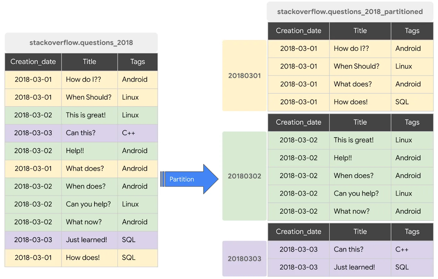
Check the previous video and also here to see an example of the performance gain.

The example SQL query can be like this:

CREATE OR REPLACE TABLE `stackoverflow.questions_2018_partitioned`
PARTITION BY
 DATE(creation_date) AS
SELECT
 *
FROM
 `bigquery-public-data.stackoverflow.posts_questions`
WHERE
 creation_date BETWEEN '2018-01-01' AND '2018-07-01';

Clustering

When a table is clustered in BigQuery, the table data is automatically organized based on the contents of one or more columns in the table’s schema. The columns you specify are used to collocate related data. Usually, high cardinality and non-temporal columns are preferred for clustering.

When data is written to a clustered table, BigQuery sorts the data using the values in the clustering columns. These values are used to organize the data into multiple blocks in BigQuery storage. The order of clustered columns determines the sort order of the data. When new data is added to a table or a specific partition, BigQuery performs automatic re-clustering in the background to restore the sort property of the table or partition. Auto re-clustering is completely free and autonomous for the users. [ source]

source

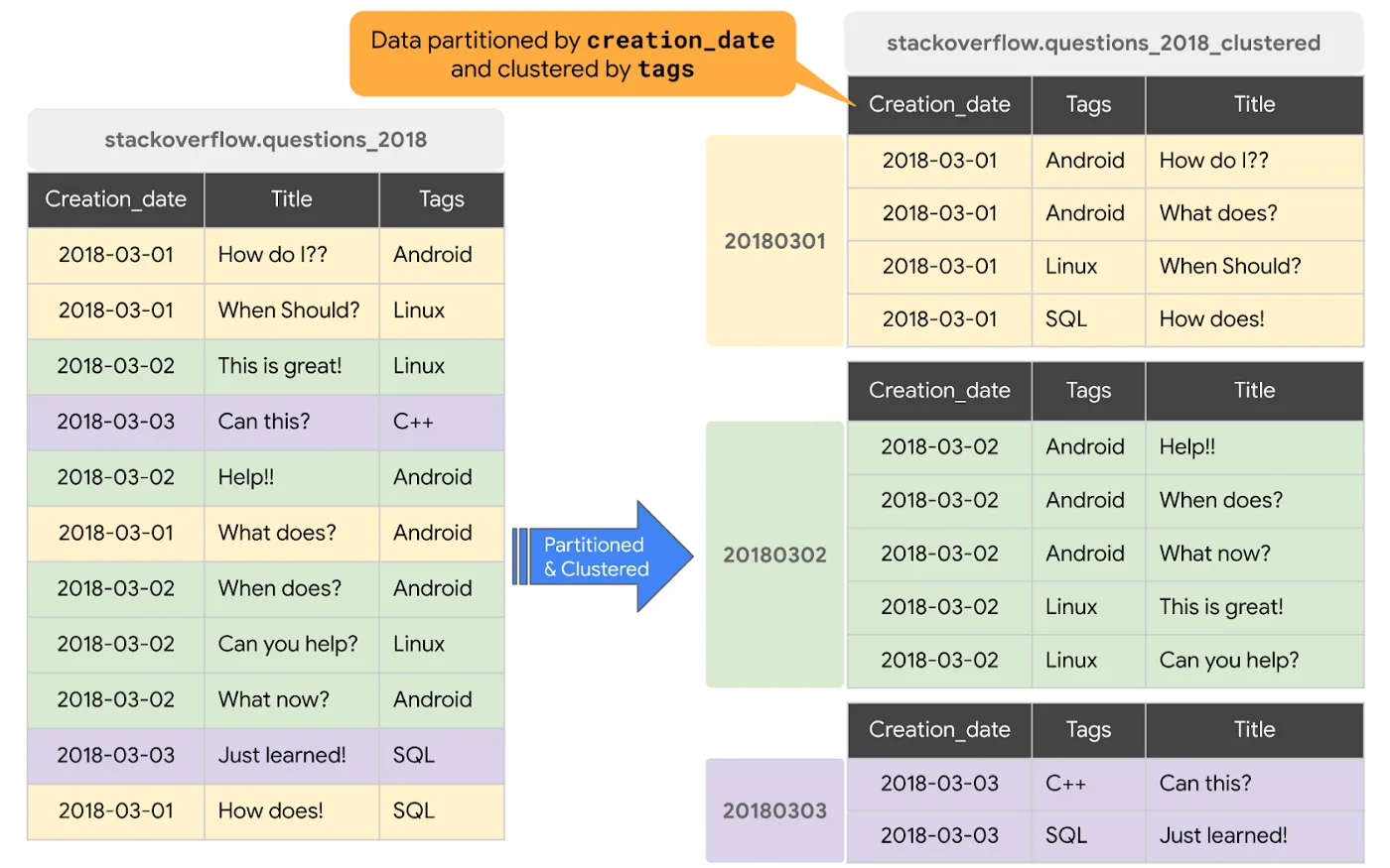
Clustering can improve the performance of certain types of queries, such as those using filter clauses and queries aggregating data. When a query containing a filter clause filters data based on the clustering columns, BigQuery uses the sorted blocks to eliminate scans of unnecessary data. When a query aggregates data based on the values in the clustering columns, performance is improved because the sorted blocks collocate rows with similar values. BigQuery supports clustering over both partitioned and non-partitioned tables. When you use clustering and partitioning together, your data can be partitioned by a DATE or TIMESTAMP column and then clustered on a different set of columns (up to four columns). [ source]

Clustered tables in BigQuery are subject to the following limitations:

• Only standard SQL is supported for querying clustered tables and for writing query results to clustered tables.
• Clustering columns must be top-level, non-repeated columns of one of the following types:
• DATE
• BOOL
• GEOGRAPHY
• INT64
• NUMERIC
• BIGNUMERIC
• STRING
• TIMESTAMP
• DATETIME
• You can specify up to four clustering columns.
• When using STRING type columns for clustering, BigQuery uses only the first 1,024 characters to cluster the data. The values in the columns can themselves be longer than 1,024.

Check the previous video and also here to see an example of the performance gain.

The example SQL query can be like this:

CREATE OR REPLACE TABLE `stackoverflow.questions_2018_clustered`
PARTITION BY
 DATE(creation_date)
CLUSTER BY
 tags AS
SELECT
 *
FROM
 `bigquery-public-data.stackoverflow.posts_questions`
WHERE
 creation_date BETWEEN '2018-01-01' AND '2018-07-01';

Check the following video to learn more:

DE Zoomcamp 3.1.2 - Partioning and Clustering

You can also check this codelab to learn more about partitioning and clustering.

Let’s now compare clustering and partitioning:

source

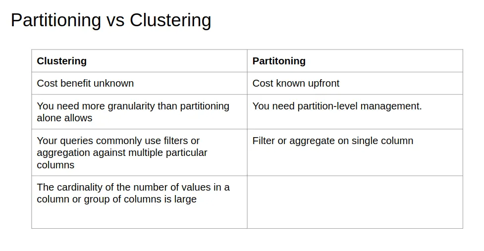
Now, let’s see when we have to choose to cluster over partitioning [ ref]:

• Partitioning results in a small amount of data per partition (approximately less than 1 GB)
• Partitioning results in a large number of partitions beyond the limits of partitioned tables
• Partitioning results in your mutation operations modifying the majority of partitions in the table frequently (for example, every few minutes)

In order to have better performance with lower cost, the following best practices in BQ are useful:

• Cost reduction

- Avoid SELECT *

- Price your queries before running them

- Use clustered or partitioned tables

- Use streaming inserts with caution

- Materialize query results in stages

• Query performance

- Filter on partitioned columns

- Denormalizing data

- Use nested or repeated columns

- Use external data sources appropriately

— Don’t use it, in case u want a high query performance

- Reduce data before using a JOIN

- Do not treat WITH clauses as prepared statements

- Avoid oversharding tables

- Avoid JavaScript user-defined functions

- Use approximate aggregation functions (HyperLogLog++)

- Order Last, for query operations to maximize performance

- Optimize your join patterns

— As a best practice, place the table with the largest number of rows first, followed by the table with the fewest rows, and then place the remaining tables by decreasing size.

Now let’s see how to load or ingest data into BigQuery and analyze them.

Direct Import (Managed Tables)

BigQuery can ingest datasets from a variety of different formats directly into its native storage. BigQuery native storage is fully managed by Google — this includes replication, backups, scaling out the size, and much more.

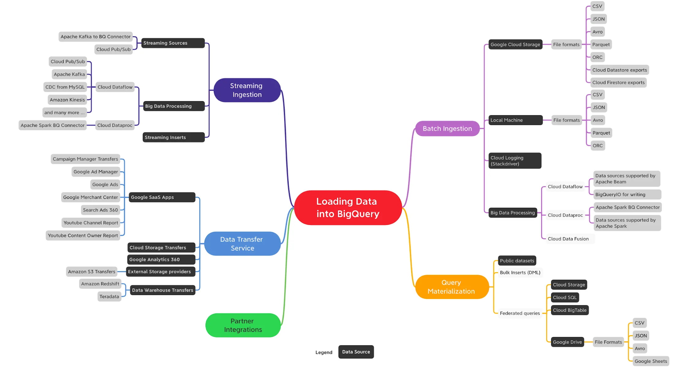
There are multiple ways to load data into BigQuery depending on data sources, data formats, load methods and use cases such as batch, streaming, or data transfer. At a high-level following are the ways you can ingest data into BigQuery:

• Batch Ingestion: Batch ingestion involves loading large, bounded, data sets that don’t have to be processed in real-time
• Streaming Ingestion: Streaming ingestion supports use cases that require analyzing high volumes of continuously arriving data with near-real-time dashboards and queries.
• Data Transfer Service (DTS): The BigQuery Data Transfer Service (DTS) is a fully managed service to ingest data from Google SaaS apps such as Google Ads, external cloud storage providers such as Amazon S3 and transfer data from data warehouse technologies such as Teradata and Amazon Redshift.
• Query Materialization: When you run queries in BigQuery their result sets can be materialized to create new tables.

source

Query without Loading (External Tables)

Using a federated query is one of the options to query external data sources directly without loading into BigQuery storage. You can query across Google services such as Google Sheets, Google Drive, Google Cloud Storage, Cloud SQL, or Cloud BigTable without having to import the data into BigQuery.

You don’t need to load data into BigQuery before running queries in the following situations:

• Public Datasets: Public datasets are datasets stored in BigQuery and shared with the public.
• Shared Datasets: You can share datasets stored in BigQuery. If someone has shared a dataset with you, you can run queries on that dataset without loading the data.
• External data sources (Federated): You can skip the data loading process by creating a table based on an external data source.

Apart from the solutions available natively in BigQuery, you can also check data integration options from Google Cloud partners who have integrated their industry-leading tools with BigQuery.

To read more, please check here.

Check the following video for BQ best practices:

DE Zoomcamp 3.2.1 - BigQuery Best Practices

Here are some example queries in BQ which shows how to do partitioning and clustering on a publicly available dataset in BQ [ ref]:

-- Query public available table
SELECT station_id, name FROM
    bigquery-public-data.new_york_citibike.citibike_stations
LIMIT 100;

-- Creating external table referring to gcs path
CREATE OR REPLACE EXTERNAL TABLE `taxi-rides-ny.nytaxi.external_yellow_tripdata`
OPTIONS (
  format = 'CSV',
  uris = ['gs://nyc-tl-data/trip data/yellow_tripdata_2019-*.csv', 'gs://nyc-tl-data/trip data/yellow_tripdata_2020-*.csv']
);

-- Check yello trip data
SELECT * FROM taxi-rides-ny.nytaxi.external_yellow_tripdata limit 10;

-- Create a non partitioned table from external table
CREATE OR REPLACE TABLE taxi-rides-ny.nytaxi.yellow_tripdata_non_partitoned AS
SELECT * FROM taxi-rides-ny.nytaxi.external_yellow_tripdata;

-- Create a partitioned table from external table
CREATE OR REPLACE TABLE taxi-rides-ny.nytaxi.yellow_tripdata_partitoned
PARTITION BY
  DATE(tpep_pickup_datetime) AS
SELECT * FROM taxi-rides-ny.nytaxi.external_yellow_tripdata;

-- Impact of partition
-- Scanning 1.6GB of data
SELECT DISTINCT(VendorID)
FROM taxi-rides-ny.nytaxi.yellow_tripdata_non_partitoned
WHERE DATE(tpep_pickup_datetime) BETWEEN '2019-06-01' AND '2019-06-30';

-- Scanning ~106 MB of DATA
SELECT DISTINCT(VendorID)
FROM taxi-rides-ny.nytaxi.yellow_tripdata_partitoned
WHERE DATE(tpep_pickup_datetime) BETWEEN '2019-06-01' AND '2019-06-30';

-- Let's look into the partitons
SELECT table_name, partition_id, total_rows
FROM `nytaxi.INFORMATION_SCHEMA.PARTITIONS`
WHERE table_name = 'yellow_tripdata_partitoned'
ORDER BY total_rows DESC;

-- Creating a partition and cluster table
CREATE OR REPLACE TABLE taxi-rides-ny.nytaxi.yellow_tripdata_partitoned_clustered
PARTITION BY DATE(tpep_pickup_datetime)
CLUSTER BY VendorID AS
SELECT * FROM taxi-rides-ny.nytaxi.external_yellow_tripdata;

-- Query scans 1.1 GB
SELECT count(*) as trips
FROM taxi-rides-ny.nytaxi.yellow_tripdata_partitoned
WHERE DATE(tpep_pickup_datetime) BETWEEN '2019-06-01' AND '2020-12-31'
  AND VendorID=1;

-- Query scans 864.5 MB
SELECT count(*) as trips
FROM taxi-rides-ny.nytaxi.yellow_tripdata_partitoned_clustered
WHERE DATE(tpep_pickup_datetime) BETWEEN '2019-06-01' AND '2020-12-31'
  AND VendorID=1;

Furthermore, if you are curious to know about the internals of BQ, you can check here, here, and also the following video.

That’s enough for this post. In the next one, I will go through how to do machine learning in BigQuery and also will review AWS Redshift.

Thank you for taking the time to read my post. If you found it helpful or enjoyable, please consider giving it a like and sharing it with your friends. Your support means the world to me and helps me to continue creating valuable content for you.