
Data Engineering: Week 3a: Data Warehouse
 Isaac Kargar6 min read
Week 3 of the Data Engineering Zoomcamp introduces analytical storage. This post uses BigQuery to explain how a warehouse stores data, how the query engine reduces work, and how data can arrive through managed and external tables.
OLTP and OLAP
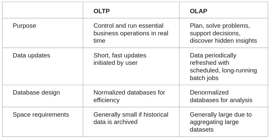
Online transaction processing (OLTP) systems record individual operations such as a payment, an order, or a change to an account. They optimise for many small reads and writes, transaction integrity, and predictable updates.
Online analytical processing (OLAP) systems answer queries across many rows. They optimise for scans, aggregations, joins, and historical analysis. A warehouse is one kind of OLAP system. A company may keep its operational database and warehouse separate so an analytical query does not compete with customer transactions.
Data warehouses
A warehouse combines data from operational systems, event streams, files, and other services into managed analytical tables. A pipeline may clean and validate data before loading it (ETL), or load the source record first and transform it inside the warehouse (ELT). The design should preserve lineage and make the quality and freshness of each table clear.
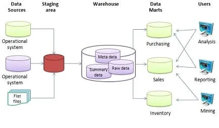
BigQuery, Amazon Redshift, and Azure Synapse are examples of managed warehouse services. This post focuses on BigQuery and uses Redshift in the next article for comparison.
BigQuery
BigQuery separates storage from the compute slots that run SQL. It can store managed tables, query supported external data sources, and run analytical SQL without a user managing database servers. The BigQuery introduction covers the service, APIs, and interfaces.
Partitioning
A partitioned table divides rows into partitions, often by ingestion time or a DATE, TIMESTAMP, or integer range column. When a query filters on the partitioning column, BigQuery can prune partitions before reading their blocks. The filter must be written so the engine can identify the relevant partitions; wrapping a column in an expression can make pruning less effective.
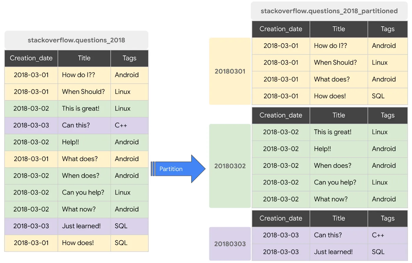
Partitioning is a storage layout and a pruning mechanism. It is not a guarantee that every query will be faster. A partitioning column should match common access patterns, and very small or very numerous partitions can create overhead. See the partitioned tables guide and querying partitioned tables.
Here is a date-partitioned table built from Stack Overflow questions:
CREATE OR REPLACE TABLE `stackoverflow.questions_2018_partitioned`
PARTITION BY DATE(creation_date) AS
SELECT *
FROM `bigquery-public-data.stackoverflow.posts_questions`
WHERE creation_date >= '2018-01-01'
  AND creation_date < '2018-07-01';
Clustering
Clustering sorts data within storage blocks using up to four configured columns. A filter on a clustered column can use block pruning, so the engine does not need to read every block in the selected partition. Clustering works on both partitioned and non-partitioned tables, and the order of the clustering columns matters.
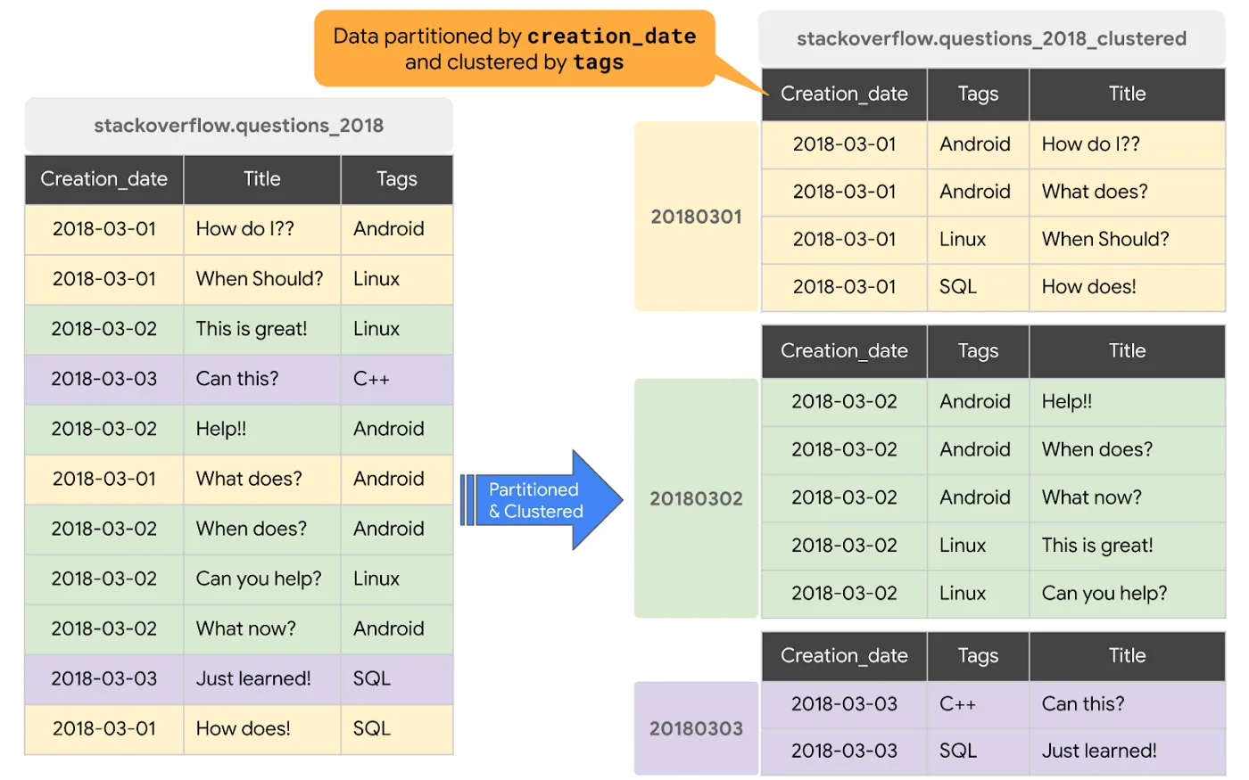
Clustering is useful when a table has repeated filters or aggregations on columns that do not make good partitions. BigQuery does not provide an exact pre-query scan estimate for a clustered table because the amount of block pruning depends on the data layout. Read the clustered tables guide and querying clustered tables for the current limits and behaviour.
CREATE OR REPLACE TABLE `stackoverflow.questions_2018_partitioned_clustered`
PARTITION BY DATE(creation_date)
CLUSTER BY tags AS
SELECT *
FROM `bigquery-public-data.stackoverflow.posts_questions`
WHERE creation_date >= '2018-01-01'
  AND creation_date < '2018-07-01';
Partitioning, clustering, and shuffle
These terms describe different mechanisms:
| Mechanism | What it does | When it helps |
|---|---|---|
| Columnar storage | Stores each column separately so a query can read only the columns it needs | Queries that select a subset of a wide table |
| Partitioning | Divides a table into coarse segments such as dates | Filters that exclude whole partitions |
| Clustering | Sorts rows into blocks within a table or partition | Filters or aggregations on recurring, higher-cardinality columns |
| Shuffle | Redistributes rows between execution workers during a query | Joins, aggregations, and other operations that need matching rows together |
Partitioning and clustering are storage-layout choices. Shuffle happens while a query runs. It is not a replacement for either layout choice.
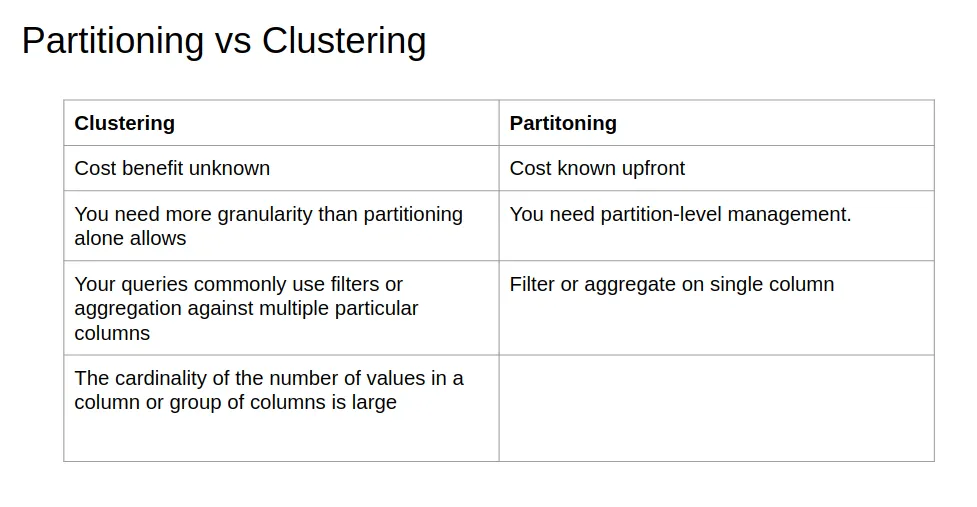
Use partitioning when the table has a strong coarse filter, such as a date range. Consider clustering when partitions would be too small or too numerous, when queries filter on several columns, or when a non-temporal column is the main access path. BigQuery can combine the two: partition by date and cluster by fields such as VendorID.
Query performance
The practical checks are simple:
- select only the columns needed by the query;
- filter on partition columns when a partitioned table is used;
- reduce rows before a large join or aggregation when that preserves the result;
- inspect the query plan and dry-run bytes before relying on a cost or timing estimate;
- avoid creating many date-sharded tables when a partitioned table provides the same access pattern.
BigQuery’s optimiser chooses a join strategy and may reorder joins. A query plan and measurements on the actual dataset are better evidence than a universal rule about join order or query speed.
Loading data into BigQuery
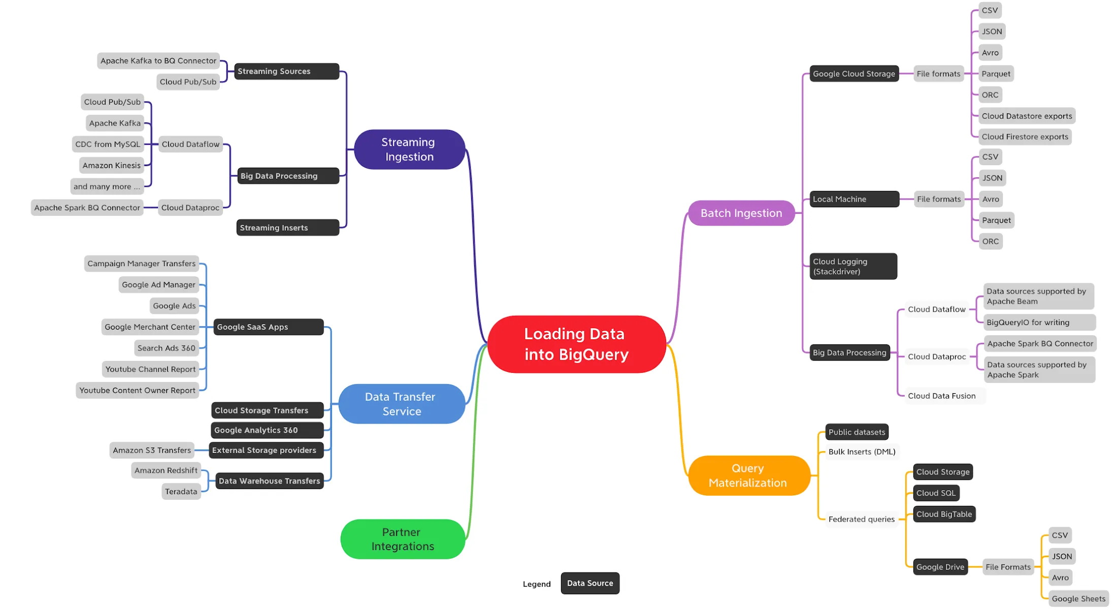
Managed tables can be loaded with a batch job, streamed into, populated from a query, or filled by a managed transfer. Batch loading is appropriate for bounded files. Streaming is appropriate when records need to become queryable with low latency and the ingestion cost and delivery guarantees fit the workload. BigQuery Data Transfer Service can copy data from supported SaaS products and storage services. The data ingestion overview lists the current choices.
External tables and federated queries
An external table gives BigQuery a table-shaped schema over data that remains in a supported external source. For example, this table reads CSV files in Cloud Storage:
CREATE OR REPLACE EXTERNAL TABLE `taxi-rides-ny.nytaxi.external_yellow_tripdata`
OPTIONS (
  format = 'CSV',
  uris = [
    'gs://nyc-tl-data/trip data/yellow_tripdata_2019-*.csv',
    'gs://nyc-tl-data/trip data/yellow_tripdata_2020-*.csv'
  ]
);
An external table is different from a federated query. A federated query uses EXTERNAL_QUERY to query supported relational systems such as Cloud SQL, AlloyDB, or Spanner and returns a temporary table to the BigQuery query. See the external data sources documentation and federated queries overview.
Public and shared BigQuery datasets are already stored in BigQuery, so they can be queried without creating a local copy. External tables and federated queries avoid a load step, but their performance, SQL support, and availability depend on the source system. Materialising a managed table can be a better choice for repeated analytical workloads.
Example: the NYC taxi dataset
The examples below use the Data Engineering Zoomcamp data warehouse materials. The numeric scan sizes are measurements from that example dataset and query plan. They are useful for seeing the direction of the effect, but they are not a promise for another table or date range.
-- Inspect an external table.
SELECT *
FROM `taxi-rides-ny.nytaxi.external_yellow_tripdata`
LIMIT 10;

-- Create a managed table without partitioning.
CREATE OR REPLACE TABLE `taxi-rides-ny.nytaxi.yellow_tripdata_non_partitioned` AS
SELECT *
FROM `taxi-rides-ny.nytaxi.external_yellow_tripdata`;

-- Create a date-partitioned managed table.
CREATE OR REPLACE TABLE `taxi-rides-ny.nytaxi.yellow_tripdata_partitioned`
PARTITION BY DATE(tpep_pickup_datetime) AS
SELECT *
FROM `taxi-rides-ny.nytaxi.external_yellow_tripdata`;

-- Create a date-partitioned and VendorID-clustered table.
CREATE OR REPLACE TABLE `taxi-rides-ny.nytaxi.yellow_tripdata_partitioned_clustered`
PARTITION BY DATE(tpep_pickup_datetime)
CLUSTER BY VendorID AS
SELECT *
FROM `taxi-rides-ny.nytaxi.external_yellow_tripdata`;

-- BigQuery can prune June partitions in this query.
SELECT DISTINCT VendorID
FROM `taxi-rides-ny.nytaxi.yellow_tripdata_partitioned`
WHERE tpep_pickup_datetime >= '2019-06-01'
  AND tpep_pickup_datetime < '2019-07-01';

-- Inspect partition metadata.
SELECT table_name, partition_id, total_rows
FROM `taxi-rides-ny.nytaxi.INFORMATION_SCHEMA.PARTITIONS`
WHERE table_name = 'yellow_tripdata_partitioned'
ORDER BY total_rows DESC;

-- A cluster filter can prune blocks within selected partitions.
SELECT COUNT(*) AS trips
FROM `taxi-rides-ny.nytaxi.yellow_tripdata_partitioned_clustered`
WHERE tpep_pickup_datetime >= '2019-06-01'
  AND tpep_pickup_datetime < '2021-01-01'
  AND VendorID = 1;
In the original comparison, the unpartitioned query scanned about 1.6 GB while the date-filtered partitioned query scanned about 106 MB. The clustered example reduced the measured scan for its query from about 1.1 GB to about 864.5 MB. Re-run a dry run or inspect the query plan after changing the table, selected columns, or date range.
The BigQuery explained series gives more detail about storage and execution.
The next article applies this warehouse to machine learning with BigQuery ML and compares it with Amazon Redshift.
Work with Nazmi
Build your AI system with Nazmi.
Tell us what you are building, what exists today, and where your team needs help.
Start a conversation or book a 20-minute call →