
Data Engineering: Week 2a: Data Ingestion
 Isaac Kargar7 min read
Week 2 of the Data Engineering Zoomcamp introduces the systems that move data from a source to a place where it can be analysed. The important distinction is between storing data, processing data, and coordinating the work that connects the two.
Data lakes
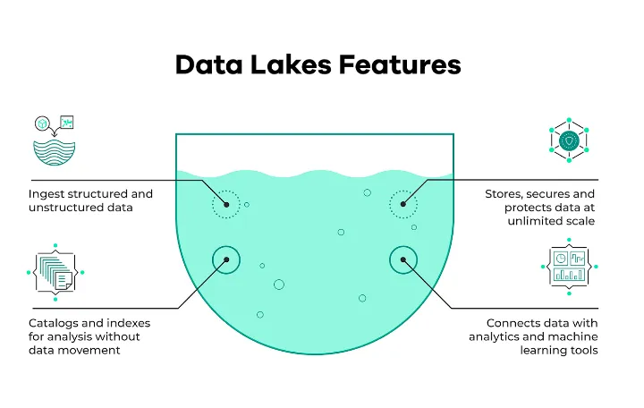
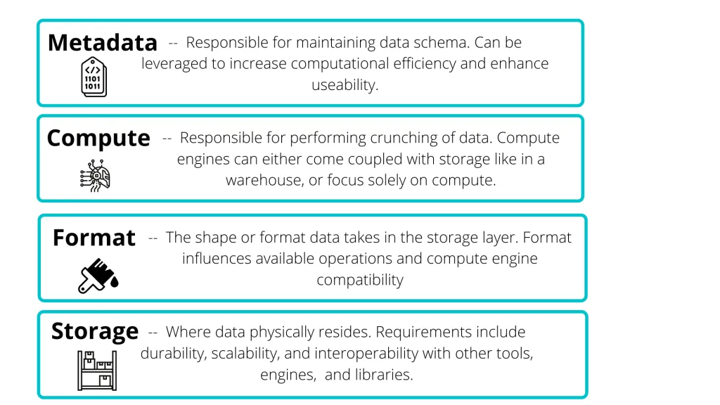
A data lake stores data in files or objects and keeps it close to its original form. The files may contain structured, semi-structured, or unstructured data. A useful lake still needs a storage layer, a format, compute that can read the data, and metadata that makes the data discoverable. The format and metadata choices determine how easy the lake is to query and govern. The lakeFS overview describes these layers and their tradeoffs.
The goal is to accept data from many systems, preserve the useful raw record, and make a governed copy available to analysts and engineers. A lake is not automatically secure, cheap, or useful. Those properties come from access controls, lifecycle policies, file formats, partitioning, catalogues, and the compute services that use it.
Data lake and data warehouse
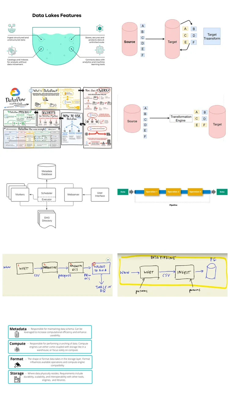
A lake and a warehouse describe different storage arrangements, but the boundary is not a rule about data types or team size. Both can store structured data, and both can support substantial workloads. A lake commonly stores files or objects in an open format and leaves more decisions about schema and processing to the consuming system. A warehouse commonly stores managed tables and provides an SQL engine, governance, and workload management for analytics.
Teams often use both. A raw event can land in object storage, be cleaned by a batch or streaming job, and then be loaded into warehouse tables for reporting. Machine learning, exploration, and operational exports may read from either system depending on latency, governance, and cost requirements.
ETL and ELT
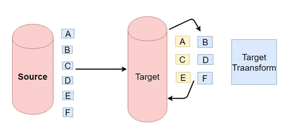
- Extract, transform, load (ETL) transforms data before loading it into the destination. This can help when the destination has a strict schema or when sensitive fields must be filtered before storage.
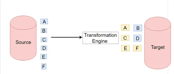
- Extract, load, transform (ELT) loads the source data first and uses the destination’s compute to transform it. This is useful when retaining the source record matters and the warehouse or lake engine can handle the transformation.
Neither method is restricted to a particular data volume or storage product. The right choice depends on the destination, data-quality requirements, governance, latency, and the cost of the transformation. The two diagrams below show the common shapes of the two approaches.
Object storage products that are often used as lake storage include Google Cloud Storage, Amazon S3, and Azure Blob Storage.
Data pipelines and orchestration
A pipeline is a sequence of work that moves data from a source through one or more processing steps to a destination. For example, one step can download a file, the next can validate and convert it, and a final step can load a table. Separating the steps lets a pipeline retry a failed upload without downloading and parsing the source again.

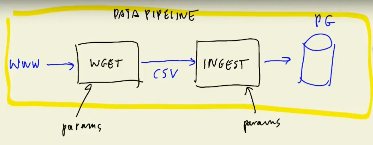
The steps in a pipeline can be independent or sequential. A directed acyclic graph (DAG) represents the dependencies: an edge from task A to task B means B can run after A succeeds. A workflow orchestrator schedules those tasks, records their state, retries failures, and exposes logs and dependencies.
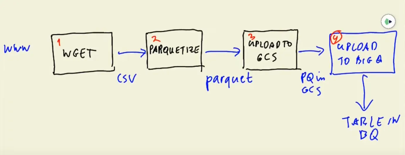
Common orchestration and processing tools include Apache Airflow, Prefect, Luigi, and Google Cloud Dataflow. They do different jobs, so comparing their names alone can be misleading.
Apache Airflow
Airflow lets us define, schedule, and monitor workflows as DAGs of tasks. Its scheduler assigns runnable tasks to an executor or workers, while the metadata database records task and DAG state. The web interface shows dependencies, logs, retries, and current runs.
Read the Airflow documentation for the current concepts and APIs.
Google Cloud Dataflow
Dataflow is a managed service for running Apache Beam pipelines. It executes batch and stream processing jobs, provisions the workers needed by those jobs, and handles the operational work of the runner. A Beam pipeline can read events, transform them, and write results to storage or a warehouse.
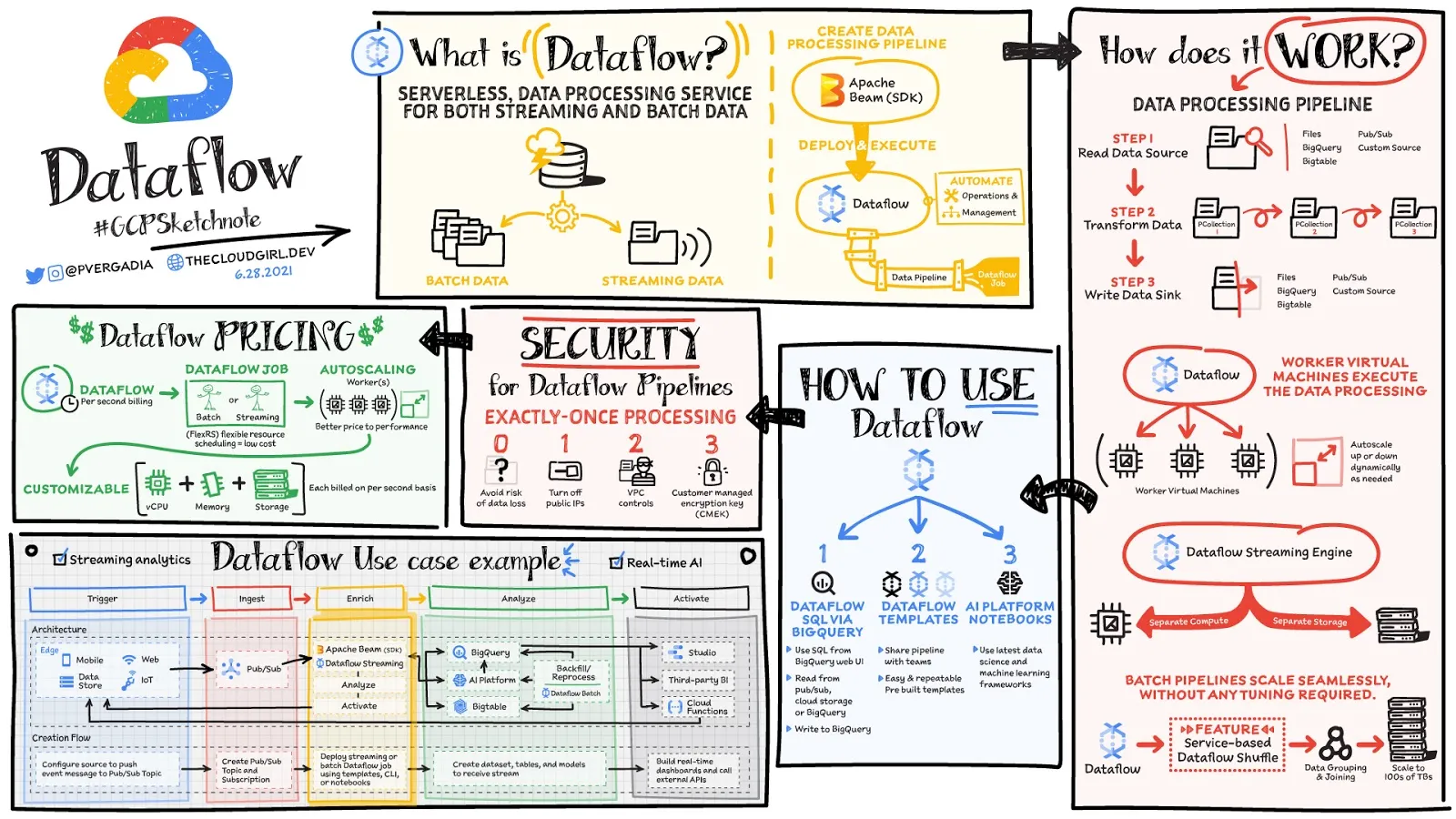
Dataflow is a processing service. An orchestrator such as Airflow can trigger and monitor a Dataflow job as one step in a larger workflow. Dataflow itself does not replace the scheduling and dependency management of that workflow. See the Dataflow overview for the batch and streaming model.
Google Cloud Composer
Cloud Composer is Google’s managed Airflow service. It provides an Airflow environment and manages its supporting infrastructure, while the DAG still describes the workflow. A DAG can coordinate BigQuery, Dataflow, Cloud Storage, or services outside Google Cloud; those services execute the individual processing jobs.
This distinction is useful when choosing between the products:
| Question | Orchestrator such as Airflow or Composer | Processor such as Dataflow |
|---|---|---|
| Main responsibility | Schedule tasks, model dependencies, retry work, and expose run state | Execute a batch or stream transformation at scale |
| Typical input | Task definitions and job parameters | A Beam pipeline and its input data |
| Typical output | A completed task, status, and logs | Transformed records written to a sink |
| Relationship | Can start and monitor a processing job | Can be one task in a larger workflow |
Run Airflow locally with Docker Compose
For this introductory example, use the Airflow Docker Compose quick-start. It provides a PostgreSQL metadata database, Redis as the Celery broker, the API server, scheduler, workers, triggerer, and an initialization service. The downloaded file defines the service set and mounts used by the quick-start.
Airflow needs a reasonable amount of memory. Allocate at least 4 GB to Docker, and more if other containers are running. Create the directories that the compose file mounts, download the file, initialize the database, and start the services:
mkdir -p dags logs plugins config
curl -LfO 'https://airflow.apache.org/docs/apache-airflow/3.3.0/docker-compose.yaml'
printf 'AIRFLOW_UID=%s\n' "$(id -u)" > .env
docker compose run airflow-cli airflow version
docker compose up airflow-init
docker compose up
Open http://localhost:8080 after the initialization service completes. The quick-start file mounts these local directories into the containers:
| Local directory | Purpose in the container |
|---|---|
./dags | DAG definitions |
./logs | Task and scheduler logs |
./plugins | Optional Airflow plugins |
./config | Optional local configuration |
The services share the PostgreSQL metadata database and Redis broker. The executor can then send a task to a worker and record its outcome. The environment is suitable for learning and local development; production deployments need an explicit security, networking, upgrade, backup, and secret-management design.
A small DAG definition shows the shape without doing heavy work while the scheduler parses the file:
from datetime import datetime

from airflow.decorators import dag, task


@dag(
    schedule="@daily",
    start_date=datetime(2024, 1, 1),
    catchup=False,
    tags=["example"],
)
def ingestion_example():
    @task
    def download() -> str:
        # Download into a durable object or shared volume in a real pipeline.
        return "raw/yellow_tripdata.csv"

    @task
    def validate(path: str) -> str:
        print(f"validating {path}")
        return path

    validate(download())


ingestion_example()
The function creates the DAG and the task functions run later in task processes. Keep the DAG module quick to import. When tasks need to exchange small values, Airflow can use XComs; large files should live in object storage or another shared data system.
This week continues with a complete Airflow ingestion walkthrough. The next post uses the same ideas to load data into a warehouse.
Work with Nazmi
Build your AI system with Nazmi.
Tell us what you are building, what exists today, and where your team needs help.
Start a conversation or book a 20-minute call →