KAN: Kolmogorov-Arnold Networks — A Short Summary

Let’s review the core concepts in the KAN paper, a new neural network architecture that sounds promising. I will review the main idea in the paper and you can check the paper for more details.

KAN vs MLP

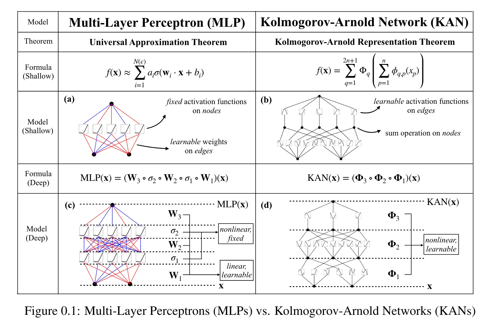
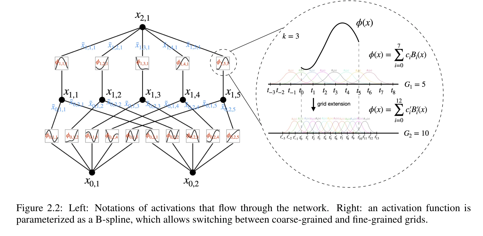
Kolmogorov-Arnold Networks (KANs) are promising alternatives to Multi-Layer Perceptrons (MLPs). Both KANs and MLPs have strong mathematical foundations: MLPs rely on the universal approximation theorem, while KANs are based on the Kolmogorov-Arnold representation theorem. Unlike MLPs, which use fixed activation functions on nodes (“neurons”), KANs employ learnable activation functions on edges (“weights”), as shown in Figure 0.1. Consequently, KANs do not have linear weight matrices; instead, each weight parameter is a learnable 1D function parameterized as a spline. KANs’ nodes merely sum incoming signals without applying any non-linearities. Essentially, according to the Kolmogrov-Arnold theorem, a multivariate function can be represented as a sum of univariate functions. Each edge connecting one neuron from one layer to a neuron in the next layer is treated as a univariate function, receiving only one input from the neuron in the previous layer. Each of these 1D functions can be parameterized as a sum of some B-spline basis functions with learnable coefficients. The output of each neuron is then computed by summing the applied activation functions to the output values of the previous layer.

There may be concerns that KANs are prohibitively expensive since each MLP’s weight parameter becomes a spline function in KANs. Fortunately, KANs typically allow for much smaller computation graphs compared to MLPs. This straightforward modification makes KANs superior (sometimes significantly!) to MLPs in terms of both model accuracy and interpretability. For interpretability, KANs can be intuitively visualized and easily interact with human users.

Splines — The Core of KAN

Splines are accurate for low-dimensional functions, easy to adjust locally, and can switch between different resolutions. However, they suffer from a significant curse of dimensionality (COD) problem due to their inability to exploit compositional structures. On the other hand, MLPs are less affected by COD because of their feature learning capabilities but are less accurate than splines in low dimensions due to their inability to optimize univariate functions. To accurately learn a function, a model must learn the compositional structure (external degrees of freedom) and approximate the univariate functions (internal degrees of freedom) well. KANs achieve this by combining MLPs on the outside and splines on the inside. Consequently, KANs can learn features (thanks to their external similarity to MLPs) and optimize these learned features with high accuracy (thanks to their internal similarity to splines).

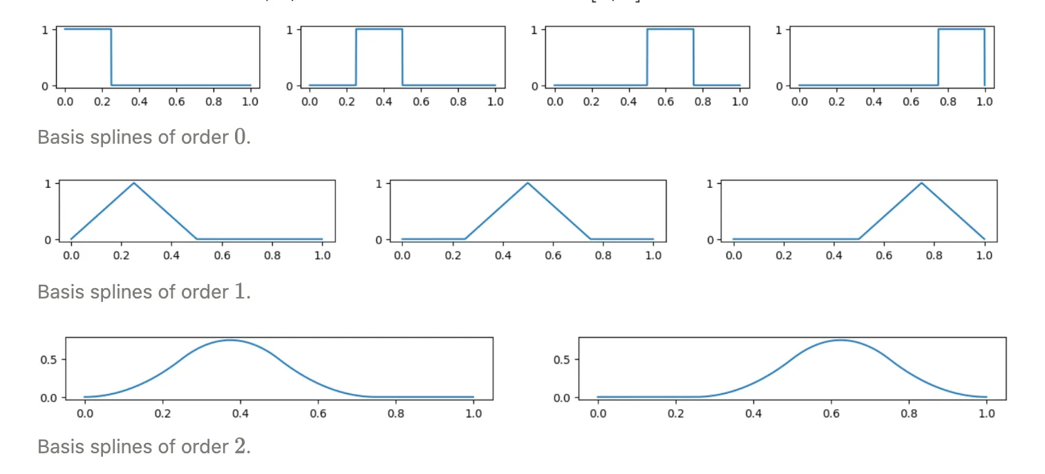
The flexibility of splines allows them to adaptively model complex relationships in the data by adjusting their shape using coefficients. The general formula for a spline can be expressed using B-splines as follows:

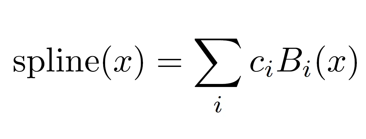
Here, spline(x) represents the spline function. The coefficients ( c_i ) are optimized during training, and ( B_i(x) ) are the B-spline basis functions defined over a grid. The grid points determine the intervals where each basis function ( B_i ) is active and significantly influences the shape and smoothness of the spline.

A spline function is defined by partitioning the domain into intervals, with each interval described by a polynomial. This ensures that the overall function remains continuous. Splines are particularly intriguing because any spline can be represented as an expansion of B-spline basis functions. Let’s visualize some B-spline basis functions of different orders:

source

To learn more about splines and B-splines, check the following resources:

• The Anatomy of a Spline | CS 4620

References

• KAN: Kolmogorov-Arnold Networks (paper, arXiv 2404.19756)
• GitHub - KindXiaoming/pykan: Kolmogorov Arnold Networks
• Hello, KAN! - Kolmogorov Arnold Network documentation

Some other references:

• Kolmogorov-Arnold Networks (KANs) | Notion
• Understanding Kolmogorov–Arnold Networks (KAN)